
Population Growth Simulator: Exponential vs Logistic Growth and Carrying Capacity
Pick a scenario, predict what the population will do, then run it and watch every birth and death while the graph draws itself. Drop droughts, disease, predators or extra food on the habitat and see why populations grow in J curves, level off in S curves, overshoot, crash and cycle.
Live math
Lab notebook
Press 📋 Record reading during a run to write the population here, with its conditions. Every factor you drop, every prediction score and every quiz result is logged too. Export a CSV of the whole run, or turn the session into a PDF lab report.
| # | Scenario / lab | Conditions | Measurement | Result |
|---|
Concept library
Click "New problem" to begin.
Click "Start quiz" for 5 questions on growth models, limiting factors, r and K, interactions, human population and sampling.
1 Overview
Every scenario is a question. Pick one from the row of cards above the lab, predict what will happen (draw it on the graph), press ▶ Run and watch: on the left the population lives in its habitat (a flask, an island, a forest, test tubes, an age pyramid), on the right its graph draws itself. The coach explains each turning point as it happens. Three modes: Simulate (free lab with learning aids and the concept library), Experiment (eight labs with a method, a conclusion and a PDF report) and Quiz (interactive challenges and a text quiz).
2 The seven scenarios
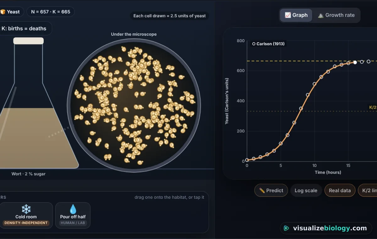
- Yeast in a flask: logistic growth to K (Carlson's 1913 data shown as circles). Change the sugar (K) or temperature (r), or close the flask so alcohol builds up.
- Design your own: pick an organism (mouse to elephant, with its r-max, strategy and survivorship type) and a model: exponential, logistic or logistic with a time lag. Set r, K and N₀.
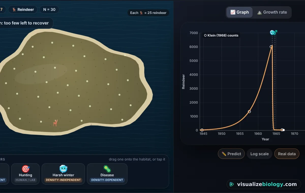
- Reindeer on an island: St Matthew Island, 1944–1980: overshoot, the record winter of 1963–64 and the crash (Klein's counts shown).
- Predator and prey: snowshoe hares and lynx; the Phase tab shows the loop.
- Two species competing: Gause's three tubes; swap the rival to see coexistence.
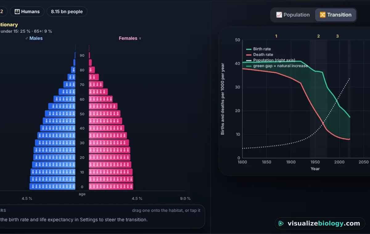
- Human population: the world from 1800 (UN milestones shown) or a model country, with the age pyramid and the Transition tab. Tick "I set the rates myself" to steer it.
- Bacteria in a flask: lag, log, stationary and death phases; use the log scale.
3 Predict, run, observe
Press ✏️ Predict under the graph (or let the page ask you when you first press Run), then draw your curve from left to right. After the run you get a match score. The graph shows K (gold dashes) and K/2, real data where there is some, and an icon for every factor you dropped. Growth rate plots dN/dt against N: for logistic growth a hump that peaks at K/2. Phase plots one species against the other with the lines where each stops growing. Hover the graph to read values; the Status button lists N, K, dN/dt, the per capita rate, the phase and the doubling time.
4 Limiting factors
Drag a factor from the tray at the bottom of the habitat (or tap it) to apply it now: drought, wildfire, harsh winter or flood (density-independent: about the same share dies at any density), disease or predators (density-dependent: a bigger share when crowded), more food or habitat loss (they change K), hunting and newcomers (human actions). With "Label factors by density" on, each chip says which kind it is: test the claim by applying it at low and at high density and comparing the share killed in the notebook.
5 Experiment mode and the lab report
Eight labs: yeast and sugar (what sets K), the doubling time of E. coli, density-dependent or independent, mark and recapture of pond snails with the Lincoln index (catch, mark, release, wait, catch again on the board), overshoot on St Matthew Island, Gause's competition, the hare and lynx cycle, and the demographic transition. Each has an aim, a method that ticks itself off as you work, a conclusion question and a PDF lab report with your readings, the habitat, the graph, calculations and limitations.
6 Quiz: interactive and text
Interactive challenges: six hands-on tasks per round from nine kinds: sketch an S curve, a J curve or a crash; tap the point of fastest growth or the carrying capacity; sort factors into density-dependent and independent (drag or tap); label the growth phases; tune r and K to hit a target; match survivorship curves; pick an age pyramid; find the predator's line; count marked snails and calculate the population. Each is marked out of 1 with partial credit, and the answer is drawn after Check. The text quiz has a practice mode with topics and worked solutions and a 5-question test with stars.
7 Units, keys and phones
SI | US switches temperatures (°C ↔ °F) and areas (km² ↔ mi², densities per km² ↔ per mi²); populations are counts in both. Keys: Space run or pause, R reset, P predict, L log scale, G switch graph, N record a reading, 1–7 scenarios, S Status. On a phone the switch at the top picks Habitat or Graph, messages appear in the strip above it, and the deck at the bottom holds Run, Settings, Factors (tap to apply), About and Aids. On a computer or tablet, Run, Step, To the end, Reset, the speed and Record reading sit under the graph.
How populations grow: exponential vs logistic growth
- Scenarios
- Yeast, a population you design, St Matthew Island reindeer, hare and lynx, Gause's Paramecium, the human population, E. coli
- You do
- Predict by drawing, run, drop limiting factors on the habitat, record readings
- It shows
- N against time with K and K/2, dN/dt against N, phase planes, age pyramids, the demographic transition
- Modes
- Simulate, Experiment (8 labs with a PDF report) and Quiz (interactive challenges + text quiz)
- Courses
- AP Biology 8.3–8.5, APES Unit 3, NGSS HS-LS2-1, AQA 3.7.4, OCR 6.3.2, IB C4.1
- Price
- Free, with no account or download; works on Chromebooks, tablets and phones
Exponential vs logistic growth (J curve vs S curve)
When food and space are unlimited, every individual can breed, so the more there are, the faster the population grows. That is exponential growth, a J curve: the AP formula sheet writes it dN/dt = rmaxN. Ten bacteria that double every 20 minutes become over a billion in nine hours. No real habitat can keep that up. As a population grows, food, water, space and nesting sites run short, so births fall and deaths rise. That is logistic growth, an S curve (sigmoid): dN/dt = rmaxN (K − N)/K. The bracket is the share of the carrying capacity still unused. Near zero the curve looks exponential, growth is fastest at N = K/2, and it stops at K.
dN/dt = rmaxN · dN/dt = rmaxN (K − N)/K · doubling time ≈ 70 ÷ growth rate (%)
| Exponential (J curve) | Logistic (S curve) | |
|---|---|---|
| Resources | Unlimited | Limited |
| Equation | dN/dt = rmaxN | dN/dt = rmaxN (K − N)/K |
| Growth rate | Keeps rising with N | Highest at K/2, zero at K |
| Per capita rate | Constant (rmax) | Falls in a straight line to 0 at K |
| Phases | Lag, then log (exponential) | Lag, log, stationary (and death in a closed culture) |
| In the simulator | Design your own → Exponential; bacteria | Yeast; Design your own → Logistic |
Carrying capacity, overshoot and dieback
The carrying capacity (K) is the largest population an environment can support over time. It is set by resources, not by the species, so it moves when the environment changes: double the sugar in the yeast flask and K doubles. A population that responds to crowding late can overshoot. In 1944, 29 reindeer were put on St Matthew Island in the Bering Sea with no wolves. By 1963 there were about 6000, eating lichen that takes decades to regrow. The record snow of winter 1963–64 hit starving animals, and by 1966 David Klein counted 42 (Journal of Wildlife Management, 1968). The simulator's island reproduces those counts.
Density-dependent and density-independent factors
Density-dependent factors hit a crowded population harder: competition for food and space, disease, parasites, predators and toxic waste. They are what bend a J curve into an S. Density-independent factors such as drought, frost, floods and fires kill about the same share at any density. In the simulator you can test this yourself: drop disease on a small population and on a crowded one and compare the share that dies.
r-selected and K-selected species
r-selected species (mice, insects, weeds) breed early and have many young with little care, so they can grow fast and crash often. K-selected species (elephants, whales, humans) have few young, care for them for a long time and stay near K. An elephant herd can grow by only about 6 % a year even with no limits; mice can quadruple. Pick each organism in "Design your own" to compare.
Survivorship curves
A survivorship curve plots how many of 1000 newborns are still alive at each age, on a log scale. Type I (humans, elephants): most live to old age. Type II (songbirds, lizards): the same chance of dying at every age, a straight line. Type III (oysters, most fish, plants): almost all die young. The interactive quiz asks you to match them.
Predator–prey cycles
Snowshoe hares and Canada lynx rise and fall in a cycle of about 10 years, seen in the Hudson's Bay Company fur records from 1845 (Elton and Nicholson, 1942). Plenty of hares feed more lynx kittens, the lynx eat the hares down, and then the lynx starve. The predator always peaks after its prey. In the Phase tab the two populations trace a loop. Giving the hares more food makes the swings bigger, not smaller (the paradox of enrichment). For whole food webs and trophic cascades, build one in Build the Food Chain.
Competition and competitive exclusion
G. F. Gause grew Paramecium aurelia and P. caudatum alone and together (1934). Alone, each reached its own carrying capacity. Together, competing for the same bacteria, P. caudatum died out. That is the competitive exclusion principle. With P. bursaria, which feeds lower in the tube, both survived (resource partitioning). The three tubes run side by side in the simulator.
Human population, age-structure diagrams and the demographic transition
About 1 billion people were alive in 1804, 2 billion in 1927 and 8 billion on 15 November 2022. The UN's World Population Prospects 2024 expects a peak of about 10.3 billion in the mid-2080s. The demographic transition explains the shape. In stage 1, high birth and death rates cancel out. In stage 2, food, clean water and vaccines cut the death rate, but the birth rate stays high. In stage 3, birth rates fall too. Stage 4 has both low, and in stage 5 there are fewer births than deaths. An age-structure diagram shows where a country is. A wide base (many children) means fast growth ahead, straight sides mean a stable population, and a narrow base means decline. A total fertility rate of about 2.1 children per woman replaces a population.
Doubling time and the rule of 70
A population growing at a steady rate doubles in about 70 ÷ (growth in % per year) years, because ln 2 ≈ 0.69. The whooping crane flock that winters in Texas has grown by about 4.2 % a year since 1938, from a low of about 15 birds to 557 in 2024–25. That is a doubling every 70 ÷ 4.2 ≈ 16.5 years.
Measuring a population: mark and recapture
To count animals that move, catch and mark M of them, release them, and later catch C and count the marked ones (R). Then N ≈ M × C ÷ R, the Lincoln index. Marking 40 snails and later catching 50, of which 8 are marked, gives about 250. The estimate assumes that marks don't come off or change behaviour, that the animals mix at random, and that nothing is born, dies or moves between the samples. The mark-and-recapture lab lets you catch, paint and recount snails on the board.
Experiments and course links
| Lab | What you find out | Course links |
|---|---|---|
| Yeast and sugar | Food sets the carrying capacity K | AP Bio 8.4; OCR 6.3.2; IB C4.1 |
| How fast do bacteria double? | Doubling time from a log graph | AP Bio 8.3; OCR 6.2.1 |
| Density-dependent or independent? | Disease vs drought at low and high density | AP Bio 8.4; APES 3.5; HS-LS2-1 |
| Mark and recapture | Lincoln index and its assumptions | AQA 3.7.4; IB C4.1 |
| Overshoot on St Matthew Island | Overshoot and dieback | APES 3.4–3.5; HS-LS2-2 |
| Gause's competition | Competitive exclusion vs resource partitioning | AP Bio 8.5; OCR 6.3.2 |
| The hare and lynx cycle | Period and lag of a predator–prey cycle | AP Bio 8.5; AQA GCSE 4.7 |
| The demographic transition | When a population grows fastest | APES 3.6–3.9 |
A population growth game with two kinds of quiz
The simulator works like a game. You draw a prediction and get a score, and you can drop disasters and see whether the population recovers. The quiz has two parts. The interactive challenges are hands-on: you sketch curves, tap the graph, drag factors into boxes, tune r and K to hit a target, read pyramids and count marked snails, with partial credit and the answer drawn for you. The text quiz asks AP-style questions with worked solutions.
Who uses this population growth simulator?
High school students in AP Biology, AP Environmental Science, GCSE, A-level and IB use it to see what the J and S curves mean, and teachers project it in class or set a lab and collect the PDF reports. It also works for introductory college ecology. It is an educational model: real populations are noisier than any simulation.
Frequently asked questions
What is the difference between exponential and logistic growth?
Exponential growth (dN/dt = rmaxN) happens when resources are unlimited: the more individuals there are, the faster the population grows, so the graph is a J curve that gets steeper and steeper. Logistic growth (dN/dt = rmaxN (K − N)/K) happens when resources are limited: growth slows as the population approaches the carrying capacity K and stops at K, so the graph is an S curve. Logistic growth is fastest when N = K/2.
What determines the carrying capacity of an environment?
The carrying capacity K is the largest population an environment can support over time. It is set by the resources and conditions the habitat provides (food, water, space, shelter, light, nesting sites) and by competition, predators, parasites and disease. K is not fixed: more food raises it and habitat loss lowers it. A population that overshoots K can damage its own food supply and crash, as the reindeer of St Matthew Island did between 1963 and 1966.
What is the difference between density-dependent and density-independent factors?
Density-dependent factors have a bigger effect when a population is crowded: competition for food and space, disease, parasites, predation and the build-up of waste. They slow growth as N rises and hold the population near K. Density-independent factors affect a population the same way at any density: weather and climate (drought, frost, heat waves), floods, fires and volcanic eruptions.
How do you estimate population size with mark and recapture?
Catch a sample of animals, count and mark them harmlessly (M), and release them. After they have mixed back in, catch a second sample (C) and count how many of them are marked (R). The population is estimated by the Lincoln index: N = M × C ÷ R. For example, 40 marked, 50 caught later of which 8 are marked gives N = 40 × 50 ÷ 8 = 250. It assumes the marks do not affect survival or catching, the animals mix at random, and there are no births, deaths or migration in between.
What is the rule of 70?
The rule of 70 estimates how long a population growing at a steady rate takes to double: doubling time ≈ 70 ÷ the growth rate in percent per year. A population growing by 2 % a year doubles in about 35 years; the whooping crane flock, growing about 4.2 % a year since 1938, doubles in about 16.5 years. It comes from ln 2 ≈ 0.693.
Explore related simulators
See who eats whom, and how removing wolves sets off a trophic cascade, in Build the Food Chain. Watch a rabbit population evolve under fox predation in the Natural Selection Simulator. Follow one cell's growth, division and the bacterial growth curve in the Virtual Bacteria Simulator, or grow a culture of amoebae in the Virtual Amoeba Simulator. Count yeast and pond life yourself in the Virtual Microscope.
Sources: OpenStax Biology 2e, chapter 45 Population and Community Ecology; Urry et al., Campbell Biology, chapter 53 Population Ecology; Carlson, Biochemische Zeitschrift 57 (1913), and Pearl, Quarterly Review of Biology 2 (1927), yeast growth; Klein, Journal of Wildlife Management 32 (1968), St Matthew Island reindeer; Gause, The Struggle for Existence (1934); Elton and Nicholson, Journal of Animal Ecology 11 (1942), the lynx cycle; United Nations, World Population Prospects 2024; US Fish and Wildlife Service, whooping crane winter counts (2025); College Board, AP Biology and AP Environmental Science Course and Exam Descriptions.
Updated