
Virtual microscope lesson plan: a 50-minute microscopy lab that works with one device per student
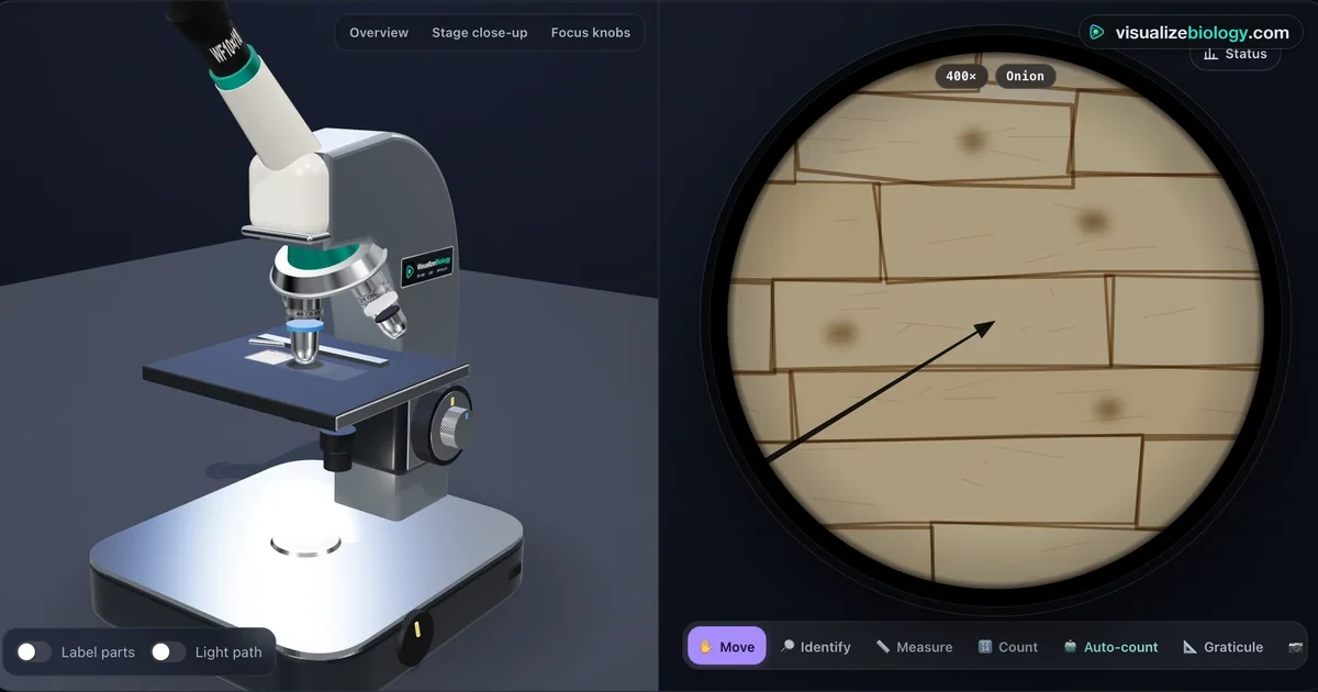
Most schools have fewer working microscopes than students, and the first microscopy lesson is the one where that hurts most. This guide is a complete 50-minute lesson built on the free Virtual Microscope. Every student focuses, measures and counts on their own screen, so the lesson can move at the pace of the class instead of the queue for the eyepiece.
It works as a pre-lab before a real practical, as a catch-up lesson for absent students, or as the whole practical where microscopes are not available. The numbers below are the ones the simulator gives, so you can check students' answers against them.
Why the first microscope lesson so often goes wrong
Picture a class of 28 with seven microscopes. Four students crowd each one. The first student turns the coarse knob at 40×, the objective hits the slide, and the coverslip cracks. The other three never get a clear image, copy a diagram from the board, and leave thinking a microscope shows you "a blurry circle".
Three skills cause almost all of that trouble, and none of them are hard. They just need practice that a crowded bench doesn't give:
- Focusing in the right order. Find the specimen at 4×, then 10×, then 40×, using only the fine knob at high power. The 40× objective's front lens sits 0.53 mm above the coverslip, so the margin for error is tiny.
- Reading the image the right way round. The image is inverted. Move the slide right and the specimen moves left.
- Knowing what magnification does and doesn't buy you. Higher power shrinks the field of view and darkens it. Detail is limited by resolution, which depends on the lens's numerical aperture, not on how big the image is.
In the simulator a cracked coverslip costs nothing. Students can make the mistake, see it, and reset, which is exactly how the skill sticks.
Before the lesson
- Devices. It runs in any modern browser, including school Chromebooks. Laptops and tablets get the 3D microscope; phones get a 2D view with the same controls. There is no login and nothing to install.
- One link for the class. Each practical has its own link, for example ?experiment=first-focus. The share bar on the tool page makes a QR code you can put on the board.
- Choose the mode. Simulate mode has two learning aids, auto-focus and auto-count. Experiment mode greys them out so students work by hand, as they would in an exam practical. For this lesson, use Experiment.
- Units. Leave the toggle on SI (µm). Students in the US who use inches for other work can switch, but microscopy answers are always marked in micrometres.
The 50-minute plan
- 0–5Predict. Ask: "A cheek cell is about 60 µm across. Will you see it at 40×? At 400×?" Students write a one-line answer and keep it for the end.
- 5–12Your first focus (5 min) and Which thread is on top? (5 min). The letter "e" slide teaches the inverted image; the crossed threads teach depth of field. At 10× only about 18 µm of the specimen is sharp at once, so students focus up and down to find which thread is highest.
- 12–24A plant cell up close (AQA GCSE RP1). Students go from 4× to 40× without losing the onion cells, find a nucleus, then drag the Measure tool along one whole cell. Expect lengths of 250 to 400 µm.
- 24–36Calibrate the eyepiece graticule. Students line up the graticule against the stage micrometer at 10×. The stage scale is 1 mm in 10 µm divisions.
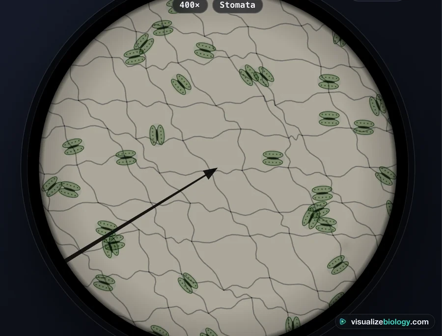
- 36–45Stomatal density. Students count every stoma in one field of view at 400× and convert the count into stomata per mm².
- 45–50Exit ticket and report. Two calculations (below), then students download the PDF lab report. It holds their settings, measurements, saved micrographs and the conclusion answers, so you have evidence of work without collecting anything.
The calculations, worked with the simulator's numbers
Calibrating the graticule
At 10×, 100 eyepiece divisions line up with 100 stage divisions. Each stage division is 10 µm, so:
At 40× the same graticule covers 4 times less specimen: 10 µm ÷ 4 = 2.5 µm
The step students most often miss is the last one. The graticule is inside the eyepiece, so its divisions don't change size when you swap objectives, but the specimen behind them does. Every objective needs its own calibration value.
Stomatal density
The field of view at 400× is 0.45 mm across, so its radius is 0.225 mm.
Density = stomata counted ÷ area = 33 ÷ 0.159 mm² ≈ 208 per mm²
Students who get 0.636 mm² have used the diameter instead of the radius. That gives an answer four times too small, and it is worth pointing out to the whole class before the exit ticket.
Real size from a drawing
Use I = A × M (image size = actual size × magnification), with both sizes in the same unit. A cell drawn 45 mm long at ×1500 is 45 mm ÷ 1500 = 0.03 mm, which is 30 µm.
- One eyepiece division is worth 10 µm at 10×. What is it worth at 40×? (2.5 µm)
- A student counts 25 stomata in a field 0.45 mm across. What is the stomatal density? (25 ÷ 0.159 mm² ≈ 157 per mm²)
Mistakes to listen for
| What students say | What is really going on | Where the simulator shows it |
|---|---|---|
| "More magnification always shows more detail." | Resolution sets the limit: 0.52 µm at 40× and 0.27 µm with the 100× oil lens. Bacteria about 1 µm long are dots at 400× and only show their shape at 1000× with oil. | The Why oil immersion? practical |
| "The image moved the wrong way, it's broken." | The objective forms an inverted image, so every movement is reversed. | Your first focus |
| "Closing the iris makes it clearer." | It raises contrast and depth of field, but lowers resolution and brightness. | The iris diaphragm trade-off |
| "I'll refocus with the big knob at 40×." | The coarse knob moves the stage far more than the 0.53 mm working distance allows. | The coach warns, and the coverslip cracks if they keep going |
Adapting it for your class
Younger or less confident students can stop after the onion practical and spend the extra time drawing what they see at 100× and 400×, with a scale bar. A-level, AP and IB students can swap the stomata count for the mitotic index of a root tip (AQA A-level RP2, AP Lab 7). Classifying 40 cells takes about 15 minutes, and the interphase-heavy result leads straight into why interphase is the longest stage. The Mitosis Simulator is a good follow-up lesson.
If your next lesson is a real practical, keep the simulator open on the board while students work at the bench. Being able to point at the "same" knob on screen saves a lot of walking round the room.
Where to go next
Questions teachers ask
Can a virtual microscope replace a real microscopy practical?
Not completely. It teaches the order of focusing, the calculations and what each control does, and it removes the queue for the eyepiece. Students still need to handle a real slide, coverslip and stain at least once. Many teachers use the simulator as the pre-lab and then run the real practical in less time.
Does it work on school Chromebooks?
Yes. It runs in the browser with no download or account. Chromebooks, laptops and tablets show the 3D microscope; phones show a 2D view with the same controls and practicals.
How do students show their work?
Each Experiment practical ends with a conclusion question, and students can download a PDF lab report with their settings, measurements, saved micrographs and answers. It can be uploaded to Google Classroom or any other learning platform.
Sources
- OpenStax, Biology 2e, section 4.1 "Studying Cells" (microscopy, magnification and resolution).
- AQA, GCSE Biology (8461) specification, required practical 1: microscopy.
- AQA, A-level Biology (7402) specification, required practical 2: the mitotic index of a root tip squash.
- Optical values (field number 18 mm, numerical apertures 0.10, 0.25, 0.65 and 1.25 oil, resolution d = 0.61λ ÷ NA) are the ones built into the Virtual Microscope and listed on its page.